(Beh et al. 2015)

The analysis identifies optimal sequences for adding to an urban water supply for a set of scenarios with differing climate change, population and discount rates. Sensitivity analysis shows how the performance of each sequence for multiple criteria varies across the scenarios, and which uncertain variables have greater influence, to inform selection of an optimal sequence plan.

Approach

The approach consists of the evaluation of the robustness of sequences of water supply augmentation options (i.e., additional options to support current water supplies) over a planning horizon to cope optimally with future conditions. The sequence of options form an adaptation pathway. As a robust decision making approach, the aim is to identify solutions able to perform well under different future conditions.

Figure 1 Beh et al. 2015

Problem framing involves defining the objectives, the planning horizon, the intervals at which new water supply options may be added, the water supply options, and constraints. Stakeholders should be involved.

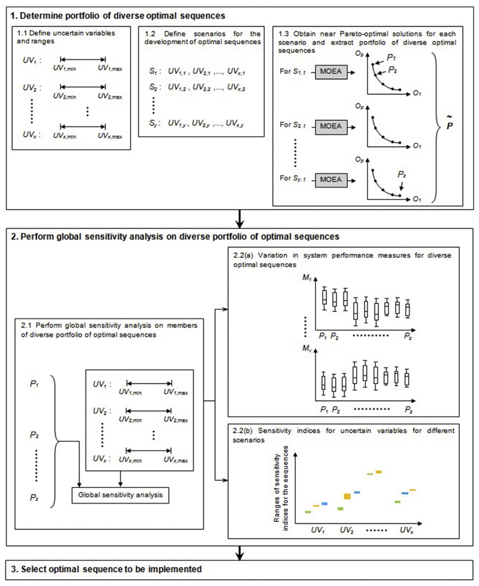
Following the problem framing stage, there are three steps:

1. Generation of a portfolio of optimal sequences:
   1. defining uncertain variables and their plausible ranges over the planning horizon
   2. defining plausible future scenarios with different combinations of values of uncertain variables
   3. generating Pareto-optimal sequences for each scenario with respect to pre-defined constraints for the different objective functions. This step may involve the use of multi-objective evolutionary algorithms (MOEAs).
2. Sensitivity analysis: evaluating the performance the Pareto-optimal sequences under a range of future conditions and the relative contribution of uncertain variables to the performance.
   • Performance metrics should include multiple specified objectives and additional measures such as reliability, resilience, or vulnerability metrics.
   • To account for variability in system states, the sensitivity analysis should be repeated for different system states for each optimal sequence.
3. Selection from the optimal sequences, which should consider:
   • trade-offs between performance objectives' absolute (e.g. average) values and variability
   • the relative contribution of uncertain variables to performance variability and consideration of the feasibility of managing those variables
   • the degree to which additional interventions could help manage constraint violations
   • the degree of adaptability of the different optimal sequences, noting that sequences that are similar at early stages provide greater adaptability

Case study details

Adelaide, the capital of South Australia, is one of the driest capital cities worldwide. It has a population of about 1.3 million with an estimated mean annual water consumption of 163 GL in 2008. The southern Adelaide water supply system (WSS) is the major water supplier, delivering 50% of the metropolitan water demand. Three reservoirs support the system supply.

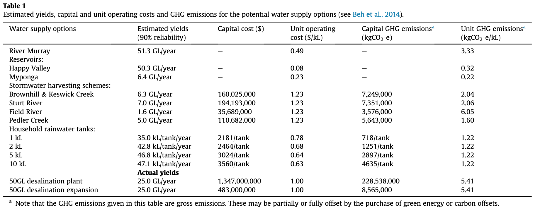
To cater for the projected water demand due to population growth and climate change, water supply augmentation sources considered include a desalination plant, diverse stormwater harvesting schemes and household rainwater tanks.

The problem formulation includes:

• Objectives: minimisation of the PV (present value) costs and PV greenhouse gas (GHG) emissions.
• Constraints: the supply capacity is greater or equal to the demand.
• Decision variables:
  • Planning horizon of 40 years
  • Decision points every 10 years (staging interval)
  • Current and future water supply sources are provided in Table 1, and the decision variable is the year in which to implement the option (Table 2). Not all of these options are independent, e.g., a specific desalination plant or stormwater harvesting scheme can only be selected once.

Table 1 Beh et al. 2015

Table 2 Beh et al. 2015

Checking constraints and calculation of objectives uses a simulation of the water supply using WaterCress (Water-Community Resource Evaluation and Simulation System).

Step 1: Determination of the portfolio of optimal sequences

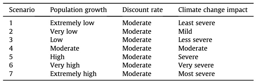
Seven scenarios are considered across three uncertain variables (Table 3). Climate change impact is represented in terms of rainfall and evaporation. Discount rates are applied to capital and operation costs and GHG emissions:

Table 3 Beh et al. 2015

These scenarios are representative of a continuum in future conditions from the best possible future conditions (scenario 1) to the worst possible (scenario 7) in terms of population and climate changes. The discount rate is kept constant here because it does not directly influence future water supply and demand.

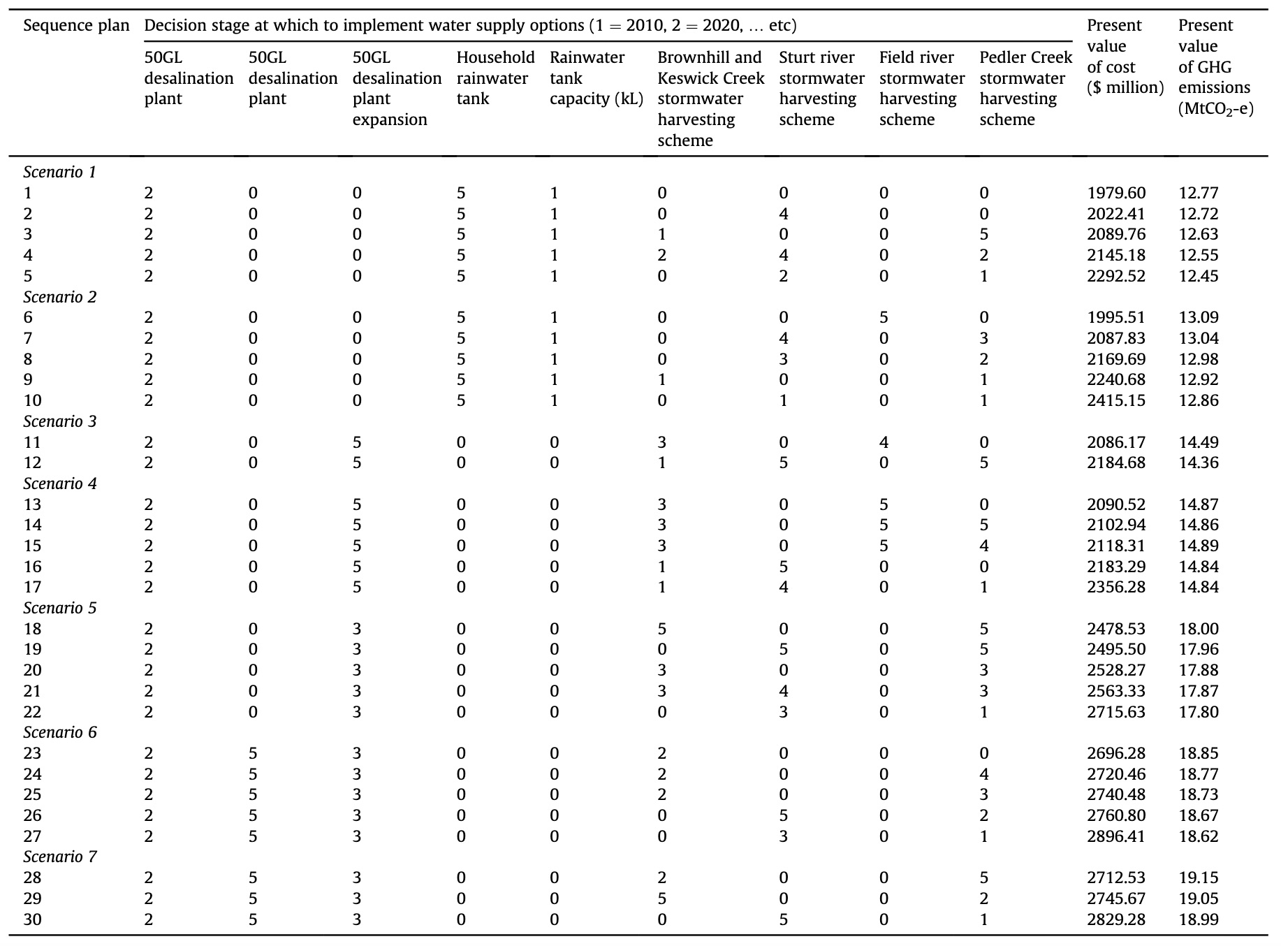
The WaterCress simulation model is used to estimate the supply, demand and costs and GHG emissions for the water supply systems under the seven scenarios, over the planning horizon, with consideration of constraints. The Water System Multiobjective Genetic Algorithm (WSMGA) is used to generate Pareto-optimal sequences. Pareto fronts are displayed in Figure 2, with selected sequences shown in Table 4.

Figure 2 Beh et al. 2015

Table 4 Beh et al. 2015

Step 2: Sensitivity analysis

Sobol's method was used for sensitivity analysis, providing sensitivity indices representing the proportion of variance in performance measures attributable to changes in single and combinations of uncertain variables.

The performance measures were the objectives, reliability (a measure of how often supply exceeds or equals demand) and vulnerability (a measure of demand shortfall).

The sensitivity analysis was repeated 20 times using stochastic daily rainfall data for the 40 year planning timeframe.

Analysis of the Sobol sensitivity indices shows that PV costs and PV GHG emissions are primarily influenced by the discount rate, with a smaller influence from population growth and climate change. Reliability and vulnerability are influenced by population growth and climate change.

Performance of optimal sequence plans across uncertain variables is presented as box-and-whiskers plots displaying the variation of the average values (over the stochastic rainfall realisations) (Figure 3).

Figure 3 Beh et al. 2015

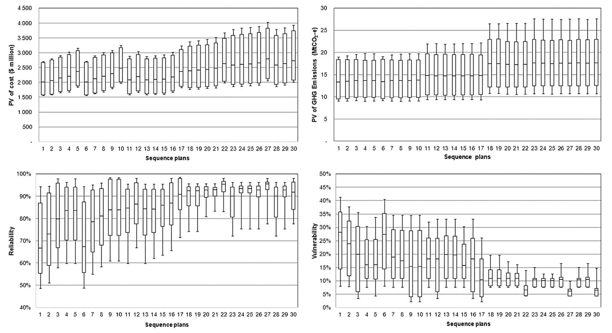
Sequence plans with higher mean values for PV costs and PV GHG emissions are generally more robust with respect to reliability and vulnerability. There is a trade-off between costs and GHG emissions on the one hand and water security (reliability and vulnerability metrics) on the other hand. Sequences 18-30 have greater reliability and less vulnerability because of early implementation of the 50 GL desalination plant expansion. Sequence 17 has less vulnerability compared to sequences 1-16 because of early implementation of stormwater schemes to reduce costs and GHG emissions.

Step 3: Selection of optimal sequence plan

An informal process is used, based on decision-makers' definition of acceptable conditions and appraisal of the following factors:

• the trade-offs between the average values and variation for the four objectives, i.e., PV costs, PV GHG emissions, reliability, vulnerability
• the relative contribution of uncertain variables (i.e., population, climate change, discount rate) to the performance results and potential for those variables to be managed
• the maximum vulnerability should be less than 27% - corresponding to what can be achieved with temporary water restrictions
• the degree of adaptability

Based on Figure 3, sequences 1-16 are excluded because the maximum vulnerability is greater than 27%. Of the remaining sequences, sequence 17 has slightly lower reliability but also lower PV costs and GHG emissions because the the 50 GL desalination expansion occurs in 2050 instead of 2030 as in sequences 18-30. The later implementation of the desalination expansion also means sequence 17 has greater adaptability. Demand restrictions have the potential to manage shortfalls due to lower reliability. Therefore, sequence 17 is selected.

Reference

Beh EHY, Maier HR, Dandy GC (2015). Scenario driven optimal sequencing under deep uncertainty. Environmental Modelling & Software 68, 181–195. doi: 10.1016/j.envsoft.2015.02.006. [Open Access version]

Also see presentation for the Queensland Water Modelling Network.

Also see Beh et al., 2015, Adaptive, multiobjective optimal sequencing approach for urban water supply augmentation under deep uncertainty